Demo

Introduction

Here is the project showcase on how I trained a clothing image classifier using Xception pre-trained CNN model. I will be using a smaller version of a bigger database to speedup my training. You can find the link to both datasets in reference.

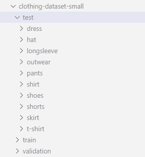
My dataset has 3085 training images, 372 validation images and 341 test images from 10 most popular classes.

What is Xception?

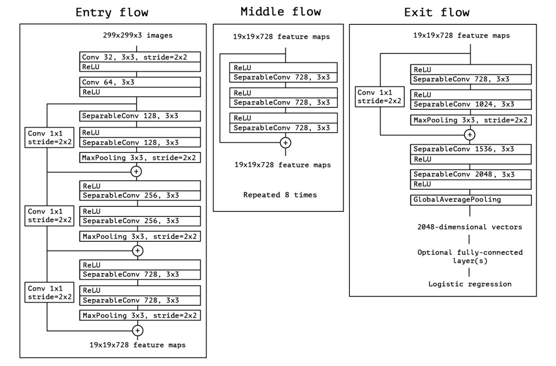
Training a performant CNN model can be a hard task due to small amount of data or lack of resources. Its possible to use pre-trained models or at least part of it, and customize it to serve our purpose. There are a lot of pre-trained models available on internet. One of such model is Xception. Following are the model specs for Xception

Size: 88 MB
Top-1 Accuracy: 79.0%
Top-5 Accuracy: 94.5%
Parameters: 22.8M
Depth: 81
CPU evaluation time: 109.4 ms
GPU evaluation time: 8.1 ms

There are other bigger models as well with better accuracy and evaluation time, but this should be fine for our experimentation and manageable for our home laptops.

Try Xception

Keras provide a way to download Xception model programmatically.

from tensorflow.keras.applications.xception import Xception

base_model = Xception(weights='imagenet', 
             input_shape=(299, 299, 3))

• By passing weights as imagenet, we tell xception class to load weights from internet. There are 2 other options. ‘none’ is used for random weights, i.e. untrained model. A path can also be passed to define a path where weights are stored for xception model architecture.
• input_shape can be anything in between (299, 299, 3) to (71, 71, 3)

Lets try to use this model and see what it predicts for an image of a t-shirt. We will get class predictions that xception model was originally trained for.

import numpy as np
from tensorflow.keras.preprocessing.image import load_img
from tensorflow.keras.applications.xception import preprocess_input

img = load_img('./tshirt.png', target_size=(299,299))
x = np.array(img)
X = np.array([x])
X = preprocess_input(X)

pred = model.predict(X)
print(pred.shape)
print(pred[0,:10])

Output

(1, 1000)
array([8.86791440e-06, 1.33468657e-05, 1.11713525e-05, 7.24550137e-06,
   3.17887934e-05, 7.48154616e-06, 2.39036472e-05, 1.15312587e-05,
   1.71842457e-05, 1.23273167e-05], dtype=float32)

• The size of prediction vector is 1000, i.e. xception original training data set had 1000 classes to predict from.
• Also the returned values are Logits and would make less sense than probability of each class. You can try applying SoftMax function to pred and see actual probabilities.

We can also use decode_predictions to do same and more.

from tensorflow.keras.applications.xception import decode_predictions
decode_predictions(pred)

Output

[[('n03595614', 'jersey', 0.97110397),
  ('n03710637', 'maillot', 0.0066445903),
  ('n04370456', 'sweatshirt', 0.00054853904),
  ('n03877472', 'pajama', 0.00053686585),
  ('n04532106', 'vestment', 0.00028699113)]]

Observe that it predicted the the image as jersey although it is a t-shirt. This does not say it is a bad model, its just that there is no class for t-shit included. The prediction by this model is based on its knowledge.

You can find the link in reference section for all the classes xception was trained on. As you might see that most of the classes (like electric_ray, hen, tree_frog, etc) are no use for us and not all of our classes are in there. So this model cannot be used as it is.

Epoch

Before we move forward we need to understand the concept of Epoch. Epoch is one iteration of learning process on whole dataset. Running multiple epochs means that model is learning on data multiple times. An optimal number of epoch can increase model performance and a large number of epoch can lead to over-fitting.

Load data

Lets load data and analyze it a bit. Following code can be used to load training data

from tensorflow.keras.preprocessing.image import ImageDataGenerator

train_gen = ImageDataGenerator(preprocessing_function=preprocess_input)
train_ds = train_gen.flow_from_directory(
    './clothing-dataset-small/train/', 
    target_size=(150,150), 
    batch_size=32,
    seed=42
)

• ImageDataGenerator is a way to load images from a filesystem. It can also be used for data augmentation. We will talk about it in next section.
• It takes preprocessing_function as input which is a function that should be applied to image data before feeding into model. Here we are passing preprocess_input which is specific to xception. We have also used it manually before while trying xception model.
• We are using smaller image size of (150, 150). This is because while experimenting we want to iterate faster and optimize our model quicker. After getting best set of hyper parameters we can retrain with larger image size.
• Batch size is number of images we should forward pass before back propagate to update weights and biases. This is important because it can help us reduce training time and generalize the model. We are starting with 32 and can optimize it later if that helps our model to improve.
• The data is shuffled before training so as to make sure that the order of images has no effect on our model. Seed is just a random number you can select to keep training same in each iteration and across different machine. Absence of this value will make each iteration to act a little different. This is not a bad thing but I personally like results that I can replicate.

Data augmentation

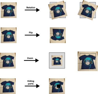
When there is limited data to train with, data can be generated by applying small transformations to existing images. This process is called data augmentation.

We should consider data augmentation in following scenarios

1. When our dataset is small.
2. When images are taken in ideal scenarios. Like properly centered and straight.
3. In real world scenario images are not that ideal specially when end user is human. This can make our model perform poor in market, if not with our dataset. Data augmentation is used to counter this shortcoming.
4. We can try this even if both of the above cases are not true for our dataset. If we can get some performance gain, it is worth the time. We can consider these transformations as hyper-parameter. If there is performance gain on applying a transformation then we should do that.

These transformation can be rotation, shift, zoom, shear, flip, hiding a random part of the image, etc.

Lets load training and validation data with data augmentation

train_gen_aug = ImageDataGenerator(preprocessing_function=preprocess_input, 
  shear_range=10.0, zoom_range=0.1, vertical_flip=True)
train_ds_aug = train_gen_aug.flow_from_directory(
  './clothing-dataset-small/train/', 
  target_size=(150,150), 
  batch_size=32,
  seed=42
)

val_gen_aug = ImageDataGenerator(preprocessing_function=preprocess_input)
val_ds_aug = val_gen_aug.flow_from_directory(
  './clothing-dataset-small/test/', 
  target_size=(150,150), 
  batch_size=32, 
  shuffle=False
)

Data augmentation is applied only to training data, not validation data. Here we are applying shear, zoom and vertical flip. In our dataset horizontal flip won’t make any difference as images are vertically symmetric and centered.

We can also use albumentations, a library solely designed for this purpose. It provides more functionalities than ImageDataGenerator.

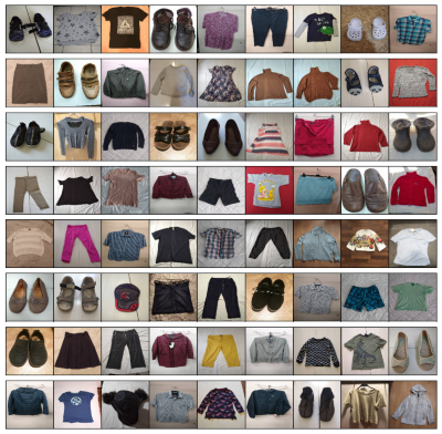
Data augmentation means we are showing more images to model. This will make model run for more epochs. Randomly selected training images.

Transfer learning

Transfer learning is a machine learning method where a model developed for a task is reused as the starting point for a model on a second task. This can be done when the data we are to train on is very small and chances is that model might over fit. This also requires that the data of the model we are trying to reuse should be somewhat similar to the data we want to use.

Example: A model trained on human faces only, cannot be reused to detect insects. Similarly a model trained to identify vehicles cannot help in identifying viruses in blood.

In this case we will be using Xception model which has been trained on 1000 classes a lot of which are clothes.

Now what we intend to do with Xception is to reuse everything before fully-connected layers. That is we will disable training for these layer parameters and treat them as a black box, or a feature extracting function.

Following code can do exactly this

base_model = Xception(weights='imagenet', 
             include_top=False, 
             input_shape=(150 ,150, 3))

base_model.trainable = False

• By passing include_top as False we can neglect fully-connected layers. The naming is like that because in Xception model layers are considered as stacked on one another, with input at bottom and target at top.
• We also need to disable xception training, as we don’t want them to change during our training. Now we will add our own fully connected layers on top of it

from tensorflow import keras

# 1
inputs = keras.Input(shape=(150,150, 3))
base = base_model(inputs, training=False)
vectors = keras.layers.GlobalAveragePooling2D()(base)
# 2
inner = keras.layers.Dense(100, activation='relu')(vectors)
# 3
drop = keras.layers.Dropout(0.5)(inner)
# 4
outputs = keras.layers.Dense(10)(drop)
# 5
model = keras.Model(inputs, outputs)

Lets look at each layer separately

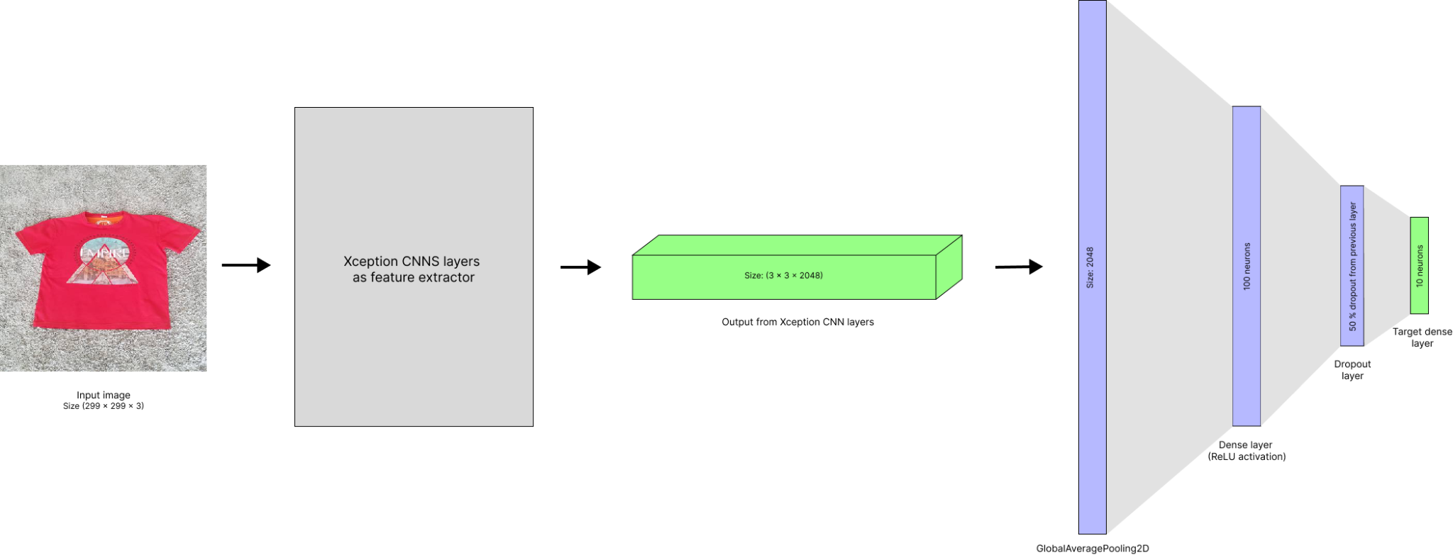
1. The shape of output from base_model (convolution part of xception) is (5, 5, 2048). This 3D data cannot be used with fully connected layers. We need to convert this into a vector.
2. So after first defining input and adding it as input to base_model, we create a GlobalAveragePooling2D layer. This will take average of output spatially, i.e. in first 2 dimensions (5, 5) and output a vector of length 2048.
3. Then we created a fully connected hidden layer with 100 neurons with ReLU activation function.
4. Next we created a dropout layer which is a good way to reduce the probability of over fitting by hiding features of image by randomly dropping fraction of nodes. This can be imagined as hiding part of image and training model to still predict it correctly. Here we are dropping out 50 % of the neurons.
5. The number of target class in our case is 10, so we define last dense layer of size 10.
6. In the end we initialized model with input and output.

Optimizer and loss function

Optimizer

Optimizers are algorithm that defines how a model going to arrive at its most optimized state. There are multiple optimizers available.

For our use case we will be using Adam optimizer which uses stochastic gradient descent to arrive at optimal state.

Optimizers require learning rate as parameter, which is how big a step model should take during training. A too big steps can overshoot model from optimal state, while smaller steps can make learning very slow.

Loss function

Loss function in a model defines how wrong the model is in its current state. Using this, model will try to improve its parameter so that loss in next iteration is smaller.

Loss function are specific to the type of model we are trying to build. Like for binary classification we can use BinaryCrossentropy. In case of multi-class classification we can use CategoricalCrossentropy loss function, which is exactly what we are going to use

optimizer = keras.optimizers.Adam(learning_rate=0.0005)
loss = keras.losses.CategoricalCrossentropy(from_logits=True)
model.compile(optimizer=optimizer, loss=loss, metrics=['accuracy'])

• In general a Softmax function is applied to produce sensible probabilities. This is something that can help human to make sense of output. But it has been noted that using softmax can produce unstable models. That is why we declared from_logits as True to disable softmax application. We have already seen how logits and softmax looks like in while trying Xception model.
• When compiling model with optimizer and loss functions we can optionally pass metrics. This tells model to keep track of custom metrics.

Training the model

Now that we have loaded training and validation data, defined model architecture and declared optimizer and loss function, we are finally ready to train our model.

history = model.fit(train_ds_aug, epochs=50, validation_data=val_ds_aug)

We can optionally pass validation data to evaluate performance of model.

This process will take time depending on resources available in our machine. If we are running this on GPU rather than CPU, our training time will reduce drastically.

As you can see, we are training our data for more epochs because of data augmentation. In absence of it, 10 epochs would have been enough.

Lets evaluate history returned by our model training.

import matplotlib.pyplot as plt
import seaborn as sns

plt.title("Accuracy")
sns.lineplot(x=history.epoch, y=history.history['accuracy'], label="train")
sns.lineplot(x=history.epoch, y=history.history['val_accuracy'], label="val")
plt.show()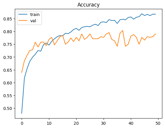

Max validation accuracy is achieved at 37 (that is 38th epoch) with training accuracy is 84.7% and validation accuracy is 80.3%.

Checkpoints and final model

Now that we are done experimenting, we are ready to train our final model on (299 x 299 x 3) image sizes. Before that lets go through another offering by keras.

Checkpoint is a callback we can pass while training to save best performant model observed till now. This is executed after each epoch. We can pass multiple checkpoints and they will be executed in order. Refer to the following code to see how its done.

checkpoint = keras.callbacks.ModelCheckpoint(
    "models/xception_v5_{epoch:02d}_{val_accuracy:.3f}.h5",
    save_best_only=True,
    monitor='val_accuracy',
    mode='max'
)

history = model.fit(train_ds_aug, epochs=50, validation_data=val_ds_aug, callbacks=[checkpoint])

• While creating ModelCheckpoint we pass formatted file path. I am saving models in models folder. I am also including epoch and validation accuracy in model file name.
• We want to save a model after each epoch if model is better that last best model. Models will be compared based on if validation accuracy is more than before.

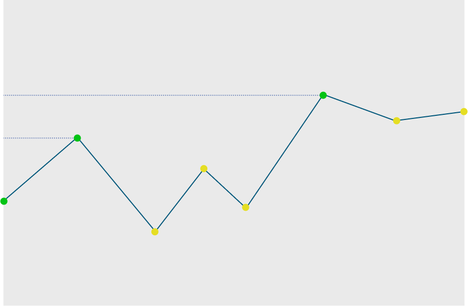
To understand it clearly lets look at figure below. As we can see models after each epoch marked green will be saved. That is total of 3 model file will be created in our filesystem.

After training our final model we see following graph

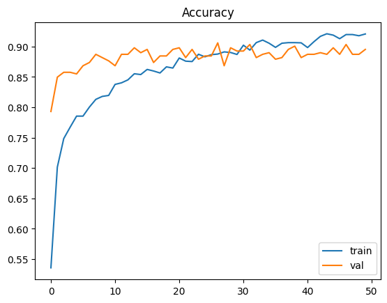
Max validation accuracy is achieved at 26 (that is 27th epoch). Training accuracy is 88.8% and validation accuracy is 90.6%. The increased accuracy is due to large image size.

As we can see validation accuracy is a little higher than train accuracy. Because training data has data augmentation enabled while validation data do not, which makes training a little harder. Its something unusual, but as they are not that different we can live with that.

Test data validation

Finally we validate our data on test dataset

test_gen_aug = ImageDataGenerator(preprocessing_function=preprocess_input)
test_ds_aug = test_gen_aug.flow_from_directory(
    './clothing-dataset-small/test/', 
    target_size=(299,299),
    batch_size=32, 
    shuffle=False
)

model.evaluate(test_ds_aug)

From here we get our test accuracy to be 86.5% which is not very far from validation accuracy.

Conclusion

So finally we have our final model. It is stored as models/xception_v5_27_0.906.h5

You might see that I am using certain values for hyper parameters. This is not coincidence. I have experimented on different values of hyper parameters and after comparing I have arrived at these values. You can find my Jupyter notebook’s link in reference section and see how I went though with it.

In my case following hyper parameters were optimal

Learning Rate : 0.0005
Hidden layer : 1 hidden layer with 100 neurons
Dropout ratio : 0.5
Data augmentations : shear, zoom and vertical flip

Using these values accuracy for my final model on (299 x 299 x 3) image sizes came up to be as following

Epoch : 26
Train accuracy : 88.8 %
Validation accuracy : 90.6 %
Test accuracy : 86.5 %

Following is the final arch diagram of our model

Reference

• Xception paper published by François Chollet
• Other pretrained models by Keras
• Small clothing dataset we used in our model
• Full clothing dataset containing 5000 images of 20 classes
• List of target classes of Xception
• List of optimizers by Keras
• List of loss functions by Keras
• My Jupyter notebook where I did actual model training