Introduction to the problem
It is quite clear that an ability of a machine to classify objects can have multiple use case in social media, online retail and video surveillance etc. Few use cases could be as following
- Face detection in social media images
- Automated image rating to safeguard underage users from explicit content
- Product type/category detection from product image
- Face classification in surveillance camera
Even though we have so many use cases, solving a Image classification problem is not very intuitive. A conventional neural network is not a practical solution as input image tend to be large, which will introduce large number of neurons in neural network layers.
An RGB image of 150 x 150 x 3 (3 being the Red, Green and Blue channels) size will require 67500 inputs, and 300 x 300 x 3 will increase this number to 270000. Even so these image size are not even practical, as images nowadays tend to be large (1920 x 1080 or higher). If we try to build a conventional neural network with this, we will end up introducing a lot of weights and biases. This will result in slow training.
Assume an input image of 300 x 300 x 3 size, number of target classes 10 and neural network of following architecture
Input -> Hidden Layer(100) -> Hidden Layer(50) -> Output(10)This will require (300 x 300 x 3) x 100 + 100 = 27000100 weights and biases in first layer, 100 x 50 + 50 = 5050 in second hidden layer and 50 * 10 + 10 = 510 in target layer. Total number of weights and biases would be 27005660 ~ 27 million. Training so many weights and biases will require a lot of time and resources.
One solution is to resize the images, i.e. resize every image to a smaller manageable size like 10 x 10. But we all know how an image looks when scaled down too much. With too much down scaling we will lose important details, and its much harder for machine to extract info from it than a human.
The solution to these problem is Convolution Neural Network (CNN). CNN is a special case of neural network which assumes input data to be an image (or 3D data). This assumptions allows us to change model architecture in such a way that the number of weights are reduced significantly.
Types of layers in Convolution Neural Network
Suppose the image size if . This can be fixed for all input images as larger images can be down scaled to fit this size. In same manner small images can be up scaled to fit this dimensions.
Convolution layer
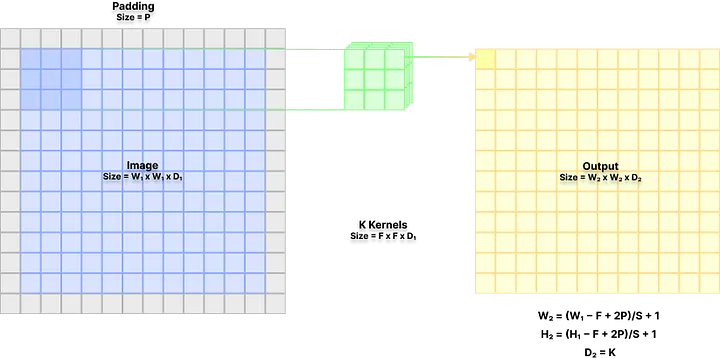
In this layer K 3D filter (kernel) of size sweep over image with a defined stride of . A zero padding of size P can also introduced to input image. This produces output of size where
This layer introduces F x F x D1 x K weights and K biases.
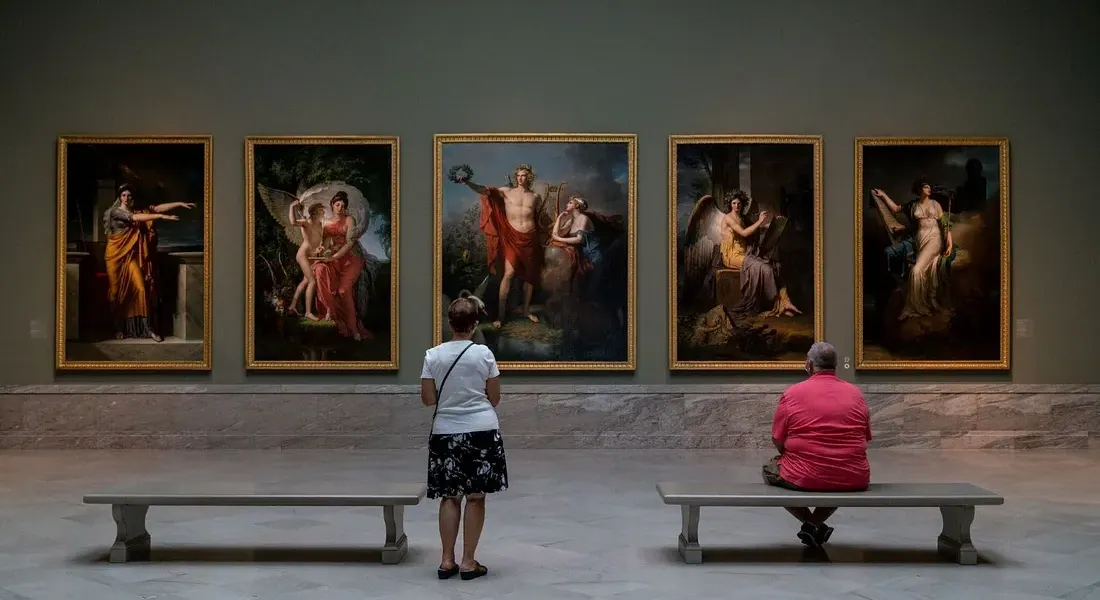
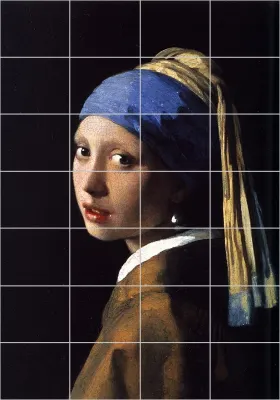
To explain this better, imagine you are looking at a famous painting in a museum. Rather than looking at it whole you might look at it one small part at a time. This is spatial extend, i.e. how much you are observing the image at a time. Stride can be understood as how fast you are iterating over the parts of the painting. After that you might observe features like eyes, nose, lips, ear, etc. and based on that your mind will register it as a face and the painting as Girl with a Pearl Earring by Johannes Vermeer.
Now following things are true after this thought experiment.
- Very large spatial extend can have negative connotations, as this means your mind is processing whole painting at once. This will be hard for your brain and will require it to work hard if you intent to do it properly.
- Very large stride might not be good as well, as you might miss important details.
ReLU layer
ReLU stands for Rectified linear Unit, where negative values are transformed to 0 and positive value are kept as it is. Following is the formula used
f(x) = max(0, x)The objective of this layer is to introduce non-linearity. In this layer the output from convolution layer is passed through ReLU activation function. This layer introduces 0 weights and biases.
Pooling layer
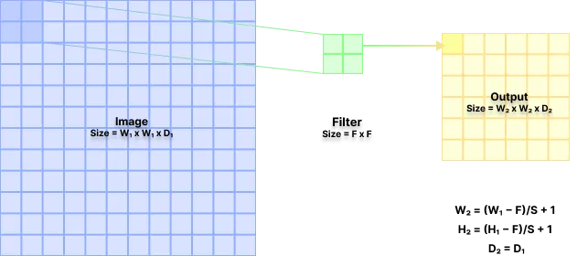
In this layer we down sample the output by sweeping a window of size with stride S and keeping only max in that window. This layer is important as it helps in reducing the chances of over-fitting and the number of parameters to be trained. For a input of size produces output of size where
This layer introduces 0 weights and biases.
Fully connected layer
Finally after we have applied Convolution, ReLU and Pooling layers certain number of times, we transform the output to a 1D vector and apply fully connected layers. This layer is conventional neural network layers.
Depending on the output size from above layers and the layers we introduce we will introduce some weights and biases, although this number is low compared to the previously introduced parameters.
Model Architecture
Our objective is to come with an optimal model architecture by defining how many layers should we have in our model and in what order. In general, a Convolution layer is always followed by a ReLU layer. This pair is then repeated multiple times before pooling layer is applied. We then repeat this multiple time and then apply Fully connected later to get desired target classes. Following is the general model architecture followed for CNN
[[Convolution layer -> ReLU layer] x N -> Pooling layer] x M
  -> [Fully connected layer -> ReLU] * L -> [Fully connected target layer]
Hyper parameters optimization
In CNN we have multiple hyper parameters we need to optimize to get a best performant model. Following are few that we should prioritize.
Size of input image size
Conventionally speaking the size of image input is kept in such a way that it is divisible by 2 many times. This is to make sure that during pooling step output layers can be feed into another and the math fits smoothly. Some of the input sizes that can be used are 32, 64, 96, 224, 384, 512, etc.
Number of filters/kernel (K)
Instinctively we start with small number of filters. Then later on we increase the number of filters as size of input decreases due to pooling. We can also increase number of filters before pooling in adjacent convolution layers + ReLU pairs.
Spatial extend of filters (F) and stride by which the filters move (S)
Most common spatial extends and stride pairs are following
Spatial extend = 3, stride = 1
Spatial extend = 5, stride = 1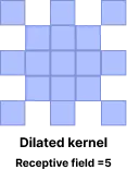
Note: There is another type of kernels being used called dilated convolution kernels. Here kernels are stacked over another with missing values.
Amount of zero padding (P)
Zero padding is used to treat edge pixels same as inner pixels. If you observe closely, filters would not cover pixels at edges properly. By introducing proper padding we ensure following 2 things
The edge pixels are treated equally and we do not loose info on edges. The spatial size of output is same as spatial size of input. Conventionally, zero padding is controlled by Spatial extend of kernels by following formula
Spatial extend of pooling filter (F) and stride by which polling filter moves (S) Generally speaking the most famous Spatial extend for pooling filter is 2 with 2 stride. In few cases spatial size of 3 with stride of 2 has also been used. This is called Overlapping pooling due to its nature.
Other than that we have to experiment with N and M defined in model architecture. Also, the number of hidden layers in fully connected layer and the number of neurons in each hidden layers should also be optimized.
Conclusion
After all this experimentation and tuning we will end up with a model that gives target output of size equal to number of classes. From here we can apply SoftMax function to get probability of each class.
That is all there is to Convolution Neural Network.
References
-
Look at CNN Explainer to visualize how it all works
-
If you wish to dig deeper take a look at Module 2 of Stanford’s course website
-
Also look at pre-trained Xception model available online.